


The opportunity
Boulder Creek Segment 2b (13th Street to the confluence with South Boulder Creek), a Class E primary-contact recreation reach under Colorado Regulation 38, has been listed as impaired for E. coli against the 126 CFU/100 mL standard since 2004. Colorado expresses that standard as a two-month geometric mean (Regulation 31, Table I, footnote 7), and Segment 2b carries no seasonal qualifier, so it applies year-round. Colorado’s first E. coli TMDL, approved by EPA Region 8 in 2011, allocated the load among the San Lazaro WWTF and four MS4 permittees, with the balance as nonpoint background. The segment remains listed as of 2024.
A large part of the difficulty is structural: contamination is episodic and flow-driven, and grab sampling captures only isolated moments, so it can miss events and gives a noisy picture of conditions. A continuous, in-situ sensor provides temporal coverage grab sampling cannot, and EPA provides a defined pathway to let that data support the recreational-use assessment. This proposal brings the two together on Segment 2b.
The regulatory pathway
The vehicle is EPA’s Site-Specific Alternative Recreational Criteria Technical Support Materials for Alternative Indicators and Methods (EPA-820-R-14-011). Under it, a state adopts an alternative indicator/method for a specified waterbody after demonstrating a consistent, predictable relationship to an EPA reference method on environmental samples, measured by an index of agreement (IA). Key features that fit Segment 2b:
- IA ≥ 0.70 against an EPA reference method permits use of the unchanged 126 CFU/100 mL criterion (no new criterion derivation).
- At least 30 paired environmental samples across the range of site conditions.
- The human-health linkage is inherited from EPA’s NEEAR epidemiology; no new epidemiological study is required.
- Single-laboratory validation is sufficient for a site-specific adoption.
Which monitoring role is which
| Monitoring role | 40 CFR 136 method required? | Approach |
|---|---|---|
| 303(d) recreational-use assessment | No | Alternative-method adoption (this proposal) |
| TMDL effectiveness / recovery-trend monitoring | No | Alternative-method adoption or screening |
| Operational screening & early warning | No | Available today |
| Numeric E. coli NPDES compliance (San Lazaro WWTF) | Yes | Outside this proposal; culture remains the reporting method |
Existing validation data
The Lume is validated for two use cases, each with its own dataset: as a grab-sample instrument that reads a collected sample, and as an in-situ field instrument deployed continuously in the creek. Both are evaluated with the statistic EPA’s framework relies on, the index of agreement (IA) on log₁₀ paired values, computed with the EPA Alternative Methods Calculator.
Use case 1 · Grab-sample instrument
Read against paired culture on controlled dilutions of Boulder Creek water. The Lume clears the IA ≥ 0.70 adoption bar against both EPA reference methods, and agrees with each more closely than the two EPA methods agree with one another.
| Comparison (reference vs. method) | n | IA | R² |
|---|---|---|---|
| Lume vs Colilert (IDEXX Quanti-Tray) | 209 | 0.96 | 0.86 |
| Lume vs membrane filtration | 206 | 0.91 | 0.70 |
| Colilert vs membrane filtration (two EPA methods) | 153 | 0.79 | 0.52 |
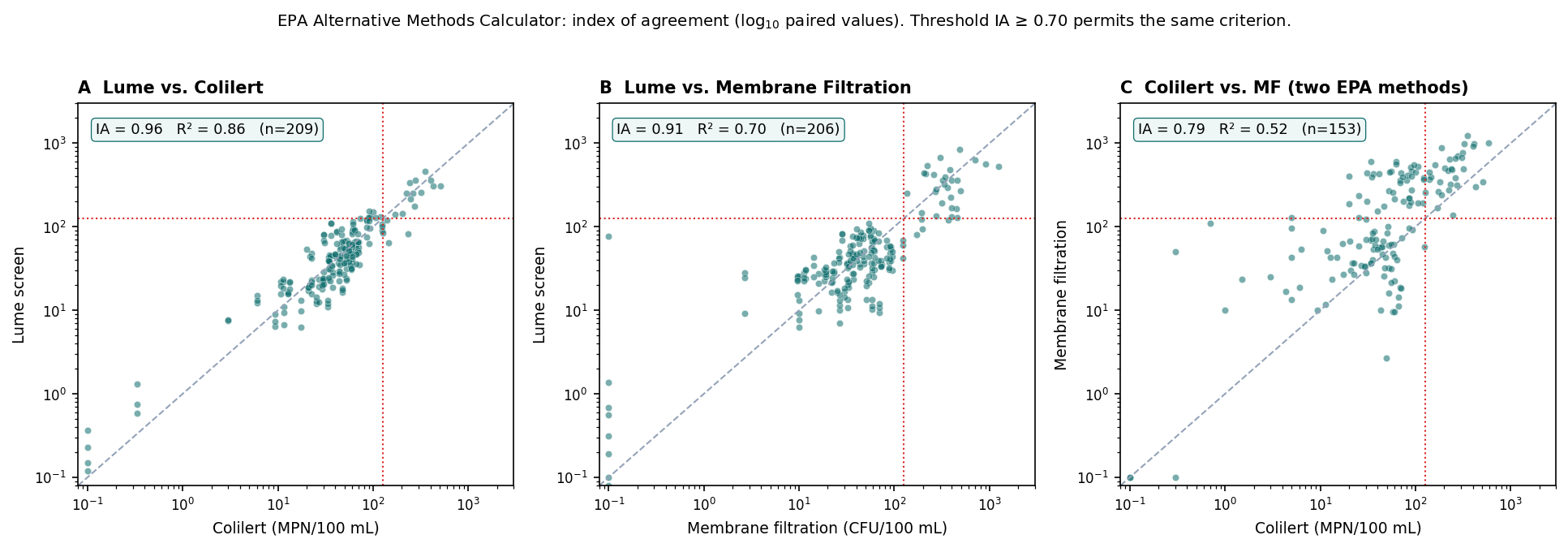
The reference methods disagree with each other more than the Lume disagrees with either. On the dedicated replicate study (n = 153), the two EPA-approved culture methods agreed at only R² = 0.52, with membrane filtration reading about 2.2× higher than Colilert; by ISO 17994 they are not equivalent to one another. The ceiling for any new method is set by how well the accepted methods agree among themselves, and the Lume meets or exceeds it.
Use case 2 · In-situ field instrument (Boulder Creek deployment)
Operated in situ on Boulder Creek with co-located Colilert grabs matched to the continuous sensor record — a harder test than reading a captured sample. On the field calibration (68 paired grabs, of which about 60 are Boulder Creek, across 8 sites, with 18 exceedances at ≥126 CFU/100 mL), the continuous model tracks Colilert at R² = 0.65 (RMSE 0.38 log₁₀), the field-only index of agreement against Colilert stays above the 0.70 adoption bar (about 0.91), and the safe-vs-unsafe classifier reaches balanced accuracy about 0.80 (sensitivity 0.79, specificity 0.80) at the 126 CFU/100 mL action limit. These figures are in-sample. Independently, a recreational deployment on the Seine and Marne (Paris) classified the 900 CFU/100 mL bathing threshold at 96.8% overall accuracy on a forward-in-time split.
In-situ field calibration and classifier detail: the Field Colilert page. Full interactive analysis (regression, Bland–Altman, classifier thresholds, per-point confidence-interval overlap, downloadable data): the Validation Data page. Framework and calculator: EPA-820-R-14-011 (PDF) · EPA Alternative Methods Calculator (Excel).
Response to the City’s questions
The City of Boulder Utilities Department put six questions to us in August 2026 while preparing to engage CDPHE on a site-specific alternative criteria proposal. They are answered here in order, so that the Division and Region 8 see the same answers the City does.
Read the draft Sampling and Analysis Plan →
1 · Method validation
Does the laboratory and field work completed to date satisfy EPA’s initial performance requirements, including specificity, sensitivity, precision, repeatability/reproducibility, accuracy, bias, and LOQ? What additional work, if any, would be needed before proceeding?
Where the requirements come from
The governing document is EPA-820-R-14-011, Site-Specific Alternative Recreational Criteria Technical Support Materials for Alternative Indicators and Methods (U.S. EPA Office of Water, Office of Science and Technology, Health and Ecological Criteria Division, December 2014) — open the PDF. It is the same document that defines this whole pathway, and it sets the bar in three places:
- Step 1, Document the Performance of the Alternative Assay. This is where the attribute list in your question comes from. The TSM draws it from EPA’s Method Validation of U.S. Environmental Protection Agency Microbiological Methods of Analysis (U.S. EPA, 2009c).
- Step 2, Gather Water Quality Data. At least 30 paired data points within the quantification limits of both assays, taken at intervals covering the range of site conditions.
- Step 3, Compare the Two Indicator/Methods. IA ≥ 0.7 against the EPA reference method, or failing that R-squared > 0.6.
Each attribute, as the TSM defines it, against what we have
| Attribute | What the TSM says | Status | Our result |
|---|---|---|---|
| Specificity | “The method’s ability to discriminate between the target organism and other (nontarget) organisms”, TN / (TN + FP), traditionally demonstrated with pure control cultures. | Documented | The construct does not transfer, by the TSM’s own design. It states the alternative may be “a different fecal indicator organism or substance” and names caffeine and detergent brighteners as examples. TLF is a bulk optical measurement of a substance, with no organism-level positive or negative call, so no control-culture TN or FP exists. What we report instead is threshold-classification specificity, 0.86 at 126 CFU/100 mL, against 0.78 for membrane filtration measured against Colilert on the same samples. |
| Sensitivity | “The proportion of target organisms that the method can detect”, TP / (TP + FN). | Documented | Same reasoning. Reported as threshold-classification sensitivity, 0.94 at 126 CFU/100 mL, balanced accuracy 0.90 (n = 209). |
| Precision and repeatability | Closeness of successive measurements under the same conditions over a short interval, as SD or %CV. | Met | About 14% relative percent difference on duplicates, against 26% or worse for Colilert duplicates. Calibration linearity R² ≥ 0.98 across 0.1–50 ppb. |
| Reproducibility | Same analyte under variable conditions, which the TSM lists as different times, analysts, reagent preparations, different instruments, and matrices. | Determined | Per-unit calibration gives each sensor its own offset and gain. Read afterwards in one shared clean-water bath, 24 units agree to 0.155 ppb (1 SD), with per-sensor bias median 0.038 ppb. That is 2% of the 7.9 ppb corresponding to the 126 CFU/100 mL criterion, and comparable to the best published field fluorimeter (UviLux, 0.17 ppb). |
| Accuracy and bias | Difference between the result and an accepted reference value. Where direct determination is unavailable, the TSM expressly permits relative recovery against an accepted reference method (ISO, 2000). | Met | Mean bias 0.00 log₁₀ against Colilert, limits of agreement ±0.42, by the relative-recovery route the TSM allows. |
| Limit of quantification | “The lowest quantity that an assay can reliably enumerate.” EPA’s worked example sets Method 1600’s LOQ at 20 colonies per membrane, the bottom of its acceptable counting range, rather than deriving it from noise. | Determined | 10 CFU/100 mL. Below it the method cannot separate contamination from its absence (62% sensitivity, 73% balanced accuracy on n = 216 paired samples); at and above it, 83–85% balanced accuracy. Independently corroborated by Sorensen et al. (2018, n = 564), who found TLF fails below 10 cfu/100 mL and called that “the limit of detection of the method, not of the instrument.” The 126 criterion sits 12.6× above this floor. |
| Agreement with the reference Step 3, the adoption test | IA ≥ 0.7, or failing that R-squared > 0.6. | Met | Cleared on both datasets, by different margins. Grab-sample comparison: IA 0.96 against Colilert and 0.91 against membrane filtration, both above the 0.79 the two EPA methods reach with each other. Continuous in-situ on Boulder Creek: IA 0.79 (n = 145, six sites). See the note below. |
What remains
Applying the LOQ costs the dataset very little. Excluding non-detects and everything below 10 CFU/100 mL leaves 326 paired observations (170 bench, 156 field) against the 30 the TSM asks for.
Three pieces of work remain, and none is a performance question:
- Confirm the LOQ in the recreational matrix. The 10 CFU/100 mL figure is established on drinking-water paired data from Rwanda and Kenya. Carrying it into recreational surface water is a cross-matrix step, and it should be reproduced on the Boulder Creek Colilert pairs before it is relied on.
- Run the official AltCalc workbook. Our index-of-agreement figures currently replicate the calculator’s arithmetic; the tool itself (EPA 821-B-21-002) should be run on the final Segment 2b dataset, which is Step 3 of the plan below. A workbook preloaded with the current indicative pairs is available for review: AltCalc workbook, Segment 2b (Excel) · paired data (CSV).
- Demonstrate precision across the concentration range on Segment 2b samples. The 14% relative percent difference on duplicates and the calibration linearity are bench figures. Reproducing them on Boulder Creek water, across the range that matters around 126 CFU/100 mL, is a duplicate-sampling design question for the SAP’s QC schedule rather than new research. Added 29 August 2026 in response to the City’s second-round question on precision.
All three are carried in the draft Sampling and Analysis Plan, Section 11, with owners, alongside the related requirement that the calibration model of record be frozen before the Step 3 analysis runs.
Three things sometimes assumed to be required here are not, on the TSM’s own terms: recovery against spiked standards (that is the ATP route, which uses spiked laboratory samples; this TSM uses unspiked environmental samples), multi-laboratory validation (Tier 1 covers a single laboratory), and any numeric threshold on the eight attributes.
2 · Study design and data adequacy
Is our current paired sampling study sufficient, or do we need to modify it to better capture the range of hydrologic, meteorological, and E. coli conditions in Boulder Creek? EPA calls for at least 30 paired observations above the LOQ and a Sampling and Analysis Plan documenting study design, representativeness, and QA/QC.
Sample count is not the constraint, even after the LOQ is applied. Taking the 10 CFU/100 mL limit from question 1, excluding non-detects, and counting only pairs at or above it leaves 326 paired observations (170 bench, 156 field) against the 30 the TSM asks for. The deployed Boulder branch is separately fitted on 145 paired grabs across 6 sites with 28 exceedances, and the method’s wider evidence base is 661 paired samples across 12 water bodies.
Note that non-detects are handled by rule rather than judgment: the AltCalc tool will not accept zero values at all, and below-detection pairs are entered blank or as BDL and excluded from the computation. So the clean-water samples in our bench ladder never enter the analysis, and the count above is what actually reaches the worksheet.
The TSM asks for samples “taken at intervals over time to cover the range of conditions at the site” and names the factors the submission must discuss: assay type, fecal sources, the age and proximity of those sources, and hydrometeorological conditions. Rather than assert that our coverage is adequate, we measured it. Each Boulder grab was matched to the discharge on its sampling day at USGS gauge 06730200 (Boulder Creek at North 75th Street) and placed in the flow distribution for the recreation season to date.
| Flow band | Grabs | Share | Exceedances ≥126 |
|---|---|---|---|
| Low (below 25th percentile) | 24 | 18% | 5 |
| Mid (25th–75th) | 60 | 44% | 7 |
| High (above 75th) | 53 | 39% | 12 |
All three flow bands are represented, and exceedances occur in every one of them. Half of all exceedances fall in the top flow quartile, but five occur at low flow, so the record is not purely event-driven and does contain dry-weather contamination.
The real gap is seasonal. The paired record runs 27 April to 3 August, concentrated in June (63 grabs) and July (48), with only six in each of April and August. There is no September or October data at all, and sampling occurred on 31 distinct days out of 118 season days elapsed. Late-season conditions, when flows recede and recreational use is still active, are unrepresented. That is what the SAP is designed to fix, and it is a scheduling question rather than a volume question. The routine and event-based schedule, and this coverage assessment, are set out in Sampling and Analysis Plan, Section 3.
3 · Documentation
Do we have, or can we readily develop, the method description and Sampling and Analysis Plan that EPA recommends? I would like to have these in a form that we could share with CDPHE relatively early in the process.
The method description exists. Method LUME-1 is drafted in EPA method-report format and available now, together with a per-unit conformance and calibration certificate that operationalizes its QC and calibration sections.
The SAP does not exist yet, and it is readily developable because the TSM supplies a template. Appendix B is an example Sampling and Analysis Plan, adapted from the City of Racine Health Department’s sampling manual, with EPA noting that “you are not limited to the elements shown in this example; you may use other SAP formats and designs.” It sets out what belongs in one: field equipment and its QC, the collection procedure, a sanitary survey at each visit, antecedent precipitation, wind, air and water temperature, and a six-hour holding time from collection to analysis.
Two related documents are named elsewhere and should be produced alongside it. The AltCalc tool’s data-documentation tab asks the submitter to record the Sampling and Analysis Plan, the Quality Assurance Project Plan, and sanitary surveys for the site, together with the sources of fecal contamination and the units of each indicator. Colorado’s 303(d) Listing Methodology separately expects analytical-method references, detection and quantitation limits, and calibration records, which Method LUME-1 and the conformance certificate already carry.
Read the draft Sampling and Analysis Plan →
It is a draft for the City to mark up before it goes to the Division. Building it now also front-loads the question above, since the SAP is where representativeness across the season and across flow conditions actually gets designed rather than described after the fact.
Method LUME-1 (PDF) · Per-Unit Conformance & Calibration Certificate (PDF) · Journal manuscript (PDF) · EPA-820-R-14-011, Appendix B (PDF)
4 · Whether the model combines indicators
One potentially important issue is EPA’s statement that the guidance does not support combining multiple indicators or methods. We should discuss whether this creates an issue for the Virridy model because it uses TLF along with turbidity and temperature to predict E. coli.
This is the most important question on the list. The TSM’s own wording answers it, on both halves.
First, a fluorescence measurement is an eligible alternative indicator. The TSM states the alternative may be “a different fecal indicator organism or substance (e.g., not enterococci or E. coli)”, and names the kind of thing it has in mind: “Additional water quality data at a site could in some cases support comparisons between different organisms or other indicator substances (e.g., caffeine, detergent brighteners).” Detergent brighteners are measured by fluorescence. A substance-based optical indicator is squarely within scope, and is not required to be organism-specific.
Second, the restriction is on tiering indicators, not on correcting a measurement. The sentence reads in full: the alternative indicator/method “is not meant to represent a combination of two or more measurements (for example, salinity and a human-specific marker in Bacteroidales used in conjunction as a tiered set of indicators).” EPA’s example is two independent measurements, each carrying its own information about contamination, combined into a tiered decision.
Temperature and turbidity are not that. Fluorescence quenches with temperature, and suspended particles scatter and attenuate light along the optical path. Both corrupt the TLF reading, and both are corrected to recover a single TLF measurement, in the same way a pH probe applies temperature compensation. Neither is an independent measure of fecal contamination, and neither carries any weight of its own in the result.
A related point we would rather raise than have asked
The value we submit as the alternative indicator is not a raw fluorescence reading. It is a calibrated estimate on the reference’s own scale, produced by a regression fitted against Colilert, and then tested for agreement against Colilert. It is fair to ask whether that builds in the agreement it goes on to demonstrate.
Three things bear on it. The pathway requires it. The index of agreement measures closeness in value, not correlation, so an indicator reported in its native units, parts per billion of tryptophan-like fluorescence, could never reach 0.7 against a reference in MPN/100 mL however well the two track. Calibration onto the reference scale is structural to the method, not a presentational choice. The TSM anticipates it, permitting recovery to be expressed relative to an accepted reference method where a direct determination against a known value is unavailable. And the independent check exists: the Seine and Marne deployment in Paris classified a different threshold, 900 CFU/100 mL, in a different matrix, on a forward-in-time split, reaching 96.8% accuracy and 94% balanced accuracy. That result is out-of-sample in the way that matters.
We would still describe the Boulder agreement figures as in-sample, and we say so in the validation section above. The honest bound on any such comparison is the one set by the reference methods themselves, which agree with each other less closely than our indicator agrees with either.
5 · Regulatory value
I would also like to better understand the end goal before we commit significant effort. Could we evaluate whether the increased sampling frequency from the sensors alone would affect Boulder Creek’s impairment status, and separately whether a site-specific criterion could provide a meaningful regulatory advantage or pathway toward delisting?
This should be tested before either party commits significant effort, and we would rather test it than assert it.
Higher sampling frequency does not automatically favour the City. A continuous record could just as easily surface exceedances that a fortnightly grab schedule was missing, and harden the listing rather than support delisting. That is a real possibility and it should be established before a proposal is drafted, not after.
The useful step is retrospective and costs nothing new in the field: the continuous record already exists, so the recreational-use assessment can be run both ways, continuous versus grab-only, under Colorado’s 303(d) Listing Methodology, to see which way the determination actually moves. We propose doing that first, and reporting the result whichever way it comes out.
- The 303(d) Listing Methodology as the Division applies it. The answer depends entirely on the decision rules: how exceedances are counted, over what assessment window, and what sample-size and confidence provisions attach. Running it against an assumed rule would produce a number worse than no number, because it would look authoritative and be wrong.
- The City’s own routine grab record for Segment 2b. Grab-only is the comparator arm, and it has to be the record an assessment would actually have used. Ours is co-located with the sensors and collected to calibrate them, which is a different sampling design and not a fair stand-in for the City’s programme.
With both in hand this is a desk analysis measured in days, not a field campaign. Without them it cannot be started, so it is the fastest item on this page to unblock.
Where the value actually sits is in measuring the standard the standard is written in. The criterion is not a single-sample number. Colorado expresses it as a geometric mean over a two-month period (Regulation 31, Table I, footnote 7), and the Division’s listing rules turn on how many samples fall inside each of those windows: two or three exceeding samples place a segment on the Monitoring and Evaluation List, five or more place it on the 303(d) List. A two-month geometric mean built on two or three grabs carries wide uncertainty, and a determination that swings on the sample count is a determination resting on the monitoring design as much as on the water. That is the concrete regulatory argument, and it holds whichever way the retrospective comes out.
So the two halves of the question separate cleanly. Whether the listing status changes is an empirical question we propose to test first, and a first cut using the Division’s published rules is now in Finding 2. Whether the assessment rests on a defensible estimate of the two-month mean is not really in doubt, and is the durable benefit.
6 · Long-term requirements
We should understand what ongoing validation and triennial reevaluation could look like so we have a sense of the long-term level of effort associated with this approach.
The triennial obligation is set by the TSM itself, and it is specific about what must be demonstrated:
So the reevaluation is not an open-ended revalidation of the instrument. It is a re-run of the Step 3 comparison on accumulated data to show the index of agreement still clears 0.7. The recurring obligations therefore fall into four parts, none of them open-ended:
| Activity | Cadence | Set by | What it involves |
|---|---|---|---|
| Per-unit recalibration and clean-water baseline | Per deployment interval | Method LUME-1 §10 | Tryptophan calibration and baseline capture per serialized unit, recording gain, intercept and detection limit on the conformance certificate. |
| Continuing accuracy samples | On the QC schedule | Method LUME-1 §9 | Paired reference samples at a defined frequency to confirm the calibration still holds in the field. |
| Ongoing paired sampling | Seasonal | SAP | Enough co-located reference grabs to detect drift and to keep extending coverage across conditions. |
| Triennial reevaluation | Every 3 years | EPA-820-R-14-011 · 40 CFR 131.20(a) | Re-run the index-of-agreement comparison on the accumulated paired record and confirm the indicator/method relationship has remained valid. Aligned to Colorado’s triennial WQS revision, so it does not add a separate cycle. |
These obligations are written into Sampling and Analysis Plan, Section 10, with the QC schedule itself in its Section 7.
The first three are recurring operational activity; the fourth is an analysis rather than a field campaign, and it reuses the record the first three already generate. Level of effort and how it is shared between the parties will be set out separately, alongside the roles still to be assigned in the Sampling and Analysis Plan.
Second round: questions of 29 August 2026
Michael Lawlor (Urban Water Quality Program Coordinator, City of Boulder Utilities) sent a further list ahead of a working session, asking that we separate what can be answered from the work completed to date from what has to go to the Division, and then consolidate the second group into a short priority list. That is how this section is organised.
Working through them against the regulations as written produced three findings that change the plan rather than just answering a question. They are set out first, because two of them correct things said earlier on this page and the third is the most time-critical item in the whole effort.
Finding 1 · Colorado does not use the criterion form the EPA pathway assumes
Colorado’s E. coli standard is not a 30-day geometric mean. Regulation 31, Table I, footnote 7 states it plainly: “Standards for E. coli are expressed as a two-month geometric mean. Site-specific or seasonal standards are also two-month geometric means unless otherwise specified.” Segment 2b (COSPBO02B) carries Recreation E with a chronic E. coli standard of 126 per 100 mL and no seasonal qualifier, so it applies in every two-month period of the year. There is no statistical threshold value in the Colorado standard at all.
The TSM, at page 24, directs the opposite: “You should use the same duration and frequency for your site-specific alternative criteria as the 2012 RWQC recommend,” which is a geometric mean over any 30-day interval plus excursions of the statistical threshold value no more than 10% of the time in that same interval.
Correction to the earlier answer. Question 5 above previously argued the regulatory value in terms of the 30-day geometric mean and the 10% excursion frequency. Those are the federal recommendation, not the standard Colorado applies to this segment, and that paragraph has been corrected. The argument survives the correction and is in fact stronger: a two-month geometric mean estimated from two or three grabs carries wider uncertainty than a 30-day one, and the Division’s own listing rules turn on how many samples fall in each two-month window.
Finding 2 · Under the Division’s own rules, this year’s record on the impaired reach attains, and the assessment unit decides it
Question 5 above said the retrospective could not start without the Division’s listing rules. We have since worked from the published methodology (Colorado’s Section 303(d) Listing Methodology, 2026 Listing Cycle, adopted March 2024; the 2028 revision, heard 9 March 2026, was limited to schedule and accessibility), which is specific enough to run. It is not a substitute for the Division confirming the applicable edition and its own practice, and it is not the full retrospective, which still needs the City’s routine grab record as the comparator arm. It is the first cut.
Method, so it can be replicated. Static two-month periods (Jan–Feb, Mar–Apr, and so on). Samples collected on the same day within the same assessment unit are reduced to their geometric mean and counted as one sample. Non-detects and zeros are converted to 1; there were none. Results above the Colilert upper limit are set to that limit; there were two. Exceedance of 126 by more than 50% in magnitude is “overwhelming evidence”. Listing follows the methodology’s Table 5: one sample no action, two or three to the Monitoring and Evaluation List, four to the 303(d) List only with overwhelming evidence, five or more indicating any degree of non-attainment straight to the 303(d) List.
Applied to the 125 Colilert grabs taken at the four stations inside the listed reach (BC-13, BC-CU, BC-30, BC-55) on 39 sampling days between 1 April and 19 August 2026:
| Assessment unit | Two-month period | Samples | Geometric mean | Outcome |
|---|---|---|---|---|
| Listed reach, pooled | Mar–Apr 2026 | 5 | 57.8 | Attains |
| Listed reach, pooled | May–Jun 2026 | 21 | 107.4 | Attains |
| Listed reach, pooled | Jul–Aug 2026 | 13 | 84.3 | Attains |
| The same data, each station treated as its own assessment unit | ||||
| BC-CU | Jul–Aug 2026 | 8 | 128.0 | 303(d) List |
| BC-30 | May–Jun 2026 | 16 | 131.0 | 303(d) List |
| BC-30 | Jul–Aug 2026 | 8 | 188.0 | 303(d) List |
| BC-55 | May–Jun 2026 | 12 | 163.0 | 303(d) List |
| BC-13, BC-Eben, BC-Can | all periods | 3–18 | 12.3–64.5 | Attain |
The reach-level result does not depend on where the reach boundary is drawn. Stations were assigned to the listed reach by position against the 13th Street crossing, so it is worth testing whether that assignment carries the conclusion. It does not. Dropping BC-13, the station closest to the upstream boundary, leaves May–June at 110.9 and July–August at 112.7, both still attaining. Pooling all six stations as a whole-segment unit gives 38.2, 59.7 and 61.6. Every reach definition we can defend attains, though the margin in the narrowest of them is 11% rather than 33%.
Three things this does not show. It covers one season of one year: there is no September, October, November, December, January or February data at all, and E. coli assessment draws on the most recent two years. Our stations were sited and sampled to calibrate sensors, not to assess a segment, so the spatial design is not the City’s. And it excludes the City’s own routine record, which is the arm that matters for a grab-versus-continuous comparison.
The part that should give everyone pause. The methodology’s sample-count ladder means a denser record removes the small-sample cushion: two or three exceeding samples land on the Monitoring and Evaluation List, but five or more land on the 303(d) List directly. Delisting is harder still, requiring at least five samples in one two-month period from the most recent two years to attain and every other two-month period with data in those two years to attain as well. A continuous record produces data in all six periods. The May–June pooled geometric mean of 107.4 sits 15% below the standard, which is not a comfortable margin. Higher frequency remains a two-sided bet, and this first cut does not change that.
Finding 3 · The Policy 25-1 clock may already be running
Commission Policy 25-1, Advancing External Proposals for Revised Water Quality Classifications and Standards (in Regulations Nos. 31-38), adopted 12 May 2025 and expiring 31 May 2028, sets the ripeness test and, more importantly here, the calendar. From 2025 the commission consolidated its scoping hearings into a single annual Triennial Review Informational Hearing (TRIH), and the policy states the deadline in the form of a worked example: for an issue to be considered at a June 2030 rulemaking hearing, the proponent should present it “no later than the TRIH in November 2028”, with the final determination made at the TRIH in November 2029.
The good news is that getting into the queue is cheap. Policy 25-1 says explicitly that “submittal of the complete data to support a proposal is not required until the proponent’s prehearing statement,” and encourages proponents to share what data they have when the issue is first raised and to “describe what they consider to be an adequate data framework.” Raising the issue at a TRIH does not commit the City to a finished dataset. It puts the issue on a published queue, gets the commission’s own view on ripeness on the record, and starts the clock rather than losing a cycle. The commission also states it may prioritise proposals that have been waiting in the queue.
We could not establish the target Regulation 38 hearing year from the public record with enough confidence to rely on it. The queue of issues and target hearing dates recorded at each TRIH is where the answer lives, and the Division can give it directly. That makes it the first question to ask, and it is the reason the sequencing below differs slightly from the proposed next steps.
Answers we can give now
Taking the questions in the order they were asked, marking each as answered here or referred to the Division.
Procedural
Next South Platte Triennial Review; is late 2028 or early 2029 still the expectation? For the Division. What we can add is Finding 3: the answer only matters because it fixes the TRIH deadline two years earlier, and if the hearing is in 2028 that deadline is this November. Ask for the hearing year and the TRIH queue entry together.
Examples of other communities that have used this pathway. For the Division, but we should not expect a long list. We could find no published instance of a state adopting a site-specific alternative indicator or method under the 2014 TSM. EPA’s own 2017 five-year review of the 2012 RWQC records that jurisdictions found the implementation documents helpful but “are struggling with development of site-specific criteria and alternative Beach Notification Thresholds.” Two consequences worth planning for: the Division will have no template to work from, and Policy 25-1 asks the Division to advise the commission on “the novelty and complexity of proposals” and whether it has the staff and expertise to review them. Novelty counts against ripeness. That is an argument for the staged engagement Michael proposes, not against the proposal.
Policy 25-1, data adequacy
How would the Division interpret data adequacy here? For the Division, but the policy’s own sub-factors are specific enough to self-assess against, and doing so shows where we actually stand:
| 25-1 | What it asks | Where we are |
|---|---|---|
| III.1.a | The record contains the data behind the conclusions, summary statistics and graphs; raw data encouraged | Met. Every figure on the validation page is backed by downloadable data. |
| III.1.b | Data files in accessible electronic form so calculations can be replicated | Met. CSV and the populated AltCalc workbook are published. |
| III.1.c | Representative, adequate in amount and type, addressing seasonal and spatial variability | The gap. Amount is not the constraint; seasonal coverage is. See the coverage answer below. |
| III.1.d | Methods discussed with the Division, CPW, EPA and stakeholders, and their input taken into account | Not yet. This is precisely the stop-gate engagement proposed, and the policy makes it a ripeness factor rather than good manners. |
| III.1.e | Data submitted for the record in the rulemaking hearing, not relied on from another regulatory context | Needs attention. Data reaching the Division through the City’s monitoring programme does not count; it has to be filed in the rulemaking record. |
| III.1.g | Data adhere to CDPHE policies and guidance for methods, collection, analysis and QA/QC where they exist | Addressed by the SAP and Method LUME-1. See the next answer for the concrete list. |
Anticipated challenges meeting CDPHE requirements for methods, collection, analysis and QA/QC. Answerable. The concrete requirements are in the Listing Methodology’s data requirements section, and most are administrative: latitude and longitude with datum, waterbody and location description, date, parameter, value, unit, the detection or reporting limit for non-detects, the method used, and submitter contact. Chemical data “should be supported by a Sampling and Analysis Plan, which identifies sampling locations, contains analytical method references, and incorporates Quality Assurance/Quality Control provisions,” and the Division may require the SAP, the QA/QC protocols and the QA/QC results. One clause speaks directly to the sensors: “Field instruments, such as multi-parameter devices, must be operated and calibrated according to manufacturer’s recommendations or other acceptable demonstrated method. Calibration information and any other documentation of accuracy may be requested by the division.” That is what the per-unit conformance and calibration certificate exists to satisfy.
The real challenge is narrower and worth naming. There is no CDPHE-approved analytical method for tryptophan-like fluorescence. The methodology says the Division “will generally accept methodologies and protocols in use by the U.S. Geological Survey, U.S. Forest Service, U.S. Bureau of Land Management, EPA, Colorado Parks and Wildlife, or others, when well documented, widely available and suitable for their intended purpose,” and that its determination on acceptability will be included in its discussion of data sources. Method LUME-1 is written to be exactly that kind of document, but acceptability is the Division’s call and is better sought early than assumed.
Timeliness
Does this proposal meet the Policy 25-1 timeliness criteria, given the emphasis on E. coli TMDLs? Answerable, and the honest answer is that timeliness is our weakest ripeness factor. The policy lists five reasons expeditious resolution could be deemed necessary. Two concern a permitted discharger unable to comply with an uncertain or infeasible standard. One concerns an attainment issue where “the proponent must demonstrate that there are no other viable pathways to address the issue and commission regulatory action is the only remaining option.” One concerns commission-set review deadlines. One concerns EPA disapproval. The best available fit is the first factor, a proposal that protects, maintains or improves water quality or existing uses in the near term, and it is an imperfect fit because changing how a segment is measured does not by itself improve water quality.
TSM Step 1, assay performance
Does the work to date meet Step 1 and allow us to proceed to Step 2? Answered in question 1 above, and that answer stands. Step 1 sets no numeric thresholds; the decision the TSM records is that “method performance is understood and deemed acceptable and rationale is provided.” All eight attributes are documented.
Can the metrics be demonstrated from paired field measurements, or must they be established in the laboratory? Answerable, and it is a mix. The TSM states that the attributes needed “can differ depending on the nature and application of the method” and that the submitter determines “the experimental designs that are best suited to evaluate performance attributes.” For accuracy and bias it expressly permits relative recovery against an accepted reference method where a direct determination against a known value is unavailable, which is a paired-field construct. Agreement, the Step 3 test, is by definition established on paired environmental samples. Precision, repeatability, calibration linearity and the limit of quantification are better established on the bench, and ours are.
Have all metrics been calculated on the Boulder Creek data, and does the dataset demonstrate precision across the full range of concentrations? Answerable, and the honest answer is no, not on Boulder Creek across the full range. The precision figure (about 14% relative percent difference on duplicates) and the calibration linearity (R² ≥ 0.98 across 0.1–50 ppb) are bench results, and the limit of quantification comes from drinking-water paired data. What Boulder Creek supplies is agreement and threshold classification. Demonstrating precision across the concentration range on Segment 2b samples is a genuine gap, and it is a third item alongside the two already listed under question 1. It is a duplicate-sampling design question, not a research question, and it belongs in the SAP’s QC schedule.
Does the Method Description Document meet the TSM requirements? Answerable. Method LUME-1 is drafted in EPA method-report format with the per-unit conformance and calibration certificate operationalising its QC and calibration sections, and both can be shared now. A consistency pass across the method, the manuscript and the figures on this site is scheduled before it goes to the Division, so that a reviewer meets one set of numbers and one description of the correction model.
TSM Step 2, water quality data
Is the SAP ready to share, and must the Division review or approve it before data count toward the 30 paired samples? Half answerable. The draft SAP exists and is shareable now. On approval: nothing in the Listing Methodology or the TSM makes Division approval a precondition for data to count. The methodology says chemical data “should be supported by” a SAP and that the Division “may require submittal of the SAP, QA/QC protocols and the results.” But Policy 25-1 III.1.d asks that the methods have been discussed with the Division and its input taken into account, which is a ripeness factor. So the practical answer is: do not wait for approval, do seek comment, and record what changed as a result. Note also that on the sample count we are already well past the TSM’s 30 paired points.
Elements CDPHE would want to see in the SAP. For the Division, and worth pre-empting: the draft is written to TSM Appendix B and separately covers every field on the Listing Methodology’s data-submittal list. Asking the Division what is missing from that starting point is a better question than asking what it wants.
Year-round sampling, or is the May to October recreation season enough? Answerable, and this is where Finding 1 bites. Segment 2b’s standard carries no seasonal qualifier, so it applies in all six two-month periods. The delisting test requires every two-month period with data in the most recent two years to attain. A grab programme that runs May to October simply generates no data in November to February, and periods without data are not assessed. A continuous sensor does not have that option: it produces data in every period, including winter, and each of those periods then has to attain. That is the sharpest practical consequence of continuous monitoring under Colorado’s rules and it needs a decision rather than a default.
How should we demonstrate that samples represent the range of hydrologic and meteorological conditions? Answerable, and the TMDL sets the frame. The 2011 TMDL is a load-duration analysis built on five flow classes defined by percent of time exceeded: high flows under 10%, moist 10–40%, mid-range 40–60%, dry 60–90%, low flow 90–100%. Demonstrating coverage against those classes uses the City’s own accepted framework rather than an ad hoc one, and it is what we have now done.
Are there gaps, and should we be targeting more wet-weather events? Answerable, and the answer is not the one the question expects. Placing each of the 125 listed-reach grabs on the flow-duration curve for USGS gauge 06730200 (Boulder Creek at North 75th Street, 9,737 daily values from 2000 to date):
| TMDL flow class | Grabs | Days | Geometric mean | TMDL required reduction |
|---|---|---|---|---|
| High flows (<10% exceeded) | 0 | 0 | — | 0.0% |
| Moist (10–40%) | 91 | 25 | 90.1 | 39.7% |
| Mid-range (40–60%) | 29 | 12 | 88.9 | 74.1% |
| Dry (60–90%) | 3 | 1 | 32.3 | 76.9% |
| Low flow (90–100%) | 2 | 1 | 19.0 | not sampled in the TMDL |
Two things follow, and they point away from storm chasing. First, no high-flow day occurred at all between 1 April and 28 August 2026: the highest daily mean in that window was 169 cfs on 30 May, which still sits in the moist class, and 96% of days in the window were moist or mid-range. The absence of wet-weather samples is a property of the year, not of the sampling schedule, and no amount of event chasing in 2026 would have fixed it. Second, the conditions the TMDL says need the largest load reductions, mid-range at 74.1% and dry at 76.9%, are the conditions we have sampled least: 12 days and 1 day respectively, against 9 dry days that actually occurred. The gap is the recession limb, not the storm peak, and the recession limb is September and October onward, which is the same seasonal gap identified in question 2. The City’s own programme, which samples weekly in September and October, covers exactly that window, which is a further reason the two records should be combined.
This also corrects the framing used earlier under question 2. Binning grabs into quartiles of the recreation season to date makes coverage look balanced by construction, because the bins are drawn from the sampled period itself. Against the flow-duration curve, which is the frame the TMDL actually uses, coverage is narrow. The earlier table is not wrong but it flatters the record, and the Division would be right to say so.
One structural point is worth making here rather than leaving implicit. A grab programme can only sample conditions it manages to be present for, which is why representativeness is hard to demonstrate and why 2026 produced no high-flow samples. A continuous record covers whatever conditions occur, by construction. That is a direct answer to the TSM’s representativeness requirement rather than an incidental benefit.
TSM Step 3, comparison and maintenance
What would CDPHE expect for the three-year re-evaluation? For the Division, with a proposal to put to it. The TSM requires only that the re-evaluation “confirm that the relationship between the indicator/methods has remained valid”, which is a re-run of the index-of-agreement comparison on accumulated data, not a repeat of Steps 1 to 3. The practical question is how many paired samples per year make that credible. Rather than ask the Division to invent a number, propose one in the SAP and ask it to confirm.
How should readings affected by sediment, turbidity or other interference be handled in QA/QC, and what other conditions should be pre-identified as grounds for exclusion? Answerable, and it is one of the more important questions on the list. The exclusion classes we already operate are: readings flagged out of water; readings outside the calibrated excitation and detector operating window; ambient light intrusion, detected on the instrument’s own dark channel; optical fouling, detected as drift on the independent time-of-flight channel rather than inferred from the fluorescence signal itself; the step change that follows a physical cleaning; and hard instrument faults. Turbidity is treated as a correction rather than an exclusion, for the reason given under question 4.
Additional questions
Is there a clear regulatory benefit, could increased TLF monitoring affect impairment status, and can this be scoped as a 2026 project? Finding 2 is the first cut and it can be scoped as a defined desk analysis. To finish it we need the City’s routine Segment 2b grab record as the comparator arm, and the Division’s confirmation of the applicable listing methodology edition and its assessment-unit practice. With those it is days of work, not a field campaign. On the second half of the question, the answer given under question 5 stands: adoption under this pathway transfers the criteria unchanged and is not a route to a looser standard. The seasonal option raised above is the one place where genuine numeric relief is contemplated by the regulations, and it is worth testing with the Division.
Does TLF coming from both viable and non-viable cells create a problem? Answerable, and the finding is more interesting than the question assumes. In field samples most tryptophan-like fluorescence is not cellular at all. Sorensen et al. (2020, Scientific Reports 10:15379) filtered 140 groundwater samples through 0.22 µm and found the majority of the signal passed through, a median of 96.9% extracellular, while at least 75% of the fluorescence from laboratory-cultured E. coli is intracellular. So the viable-versus-non-viable distinction is not the axis the measurement sits on. TLF is a bulk optical measurement of a substance and was never proposed as a cell count, which is exactly the case the TSM contemplates when it names caffeine and detergent brighteners, substances with no viability at all, as candidate alternative indicators. What has to be demonstrated is agreement with the reference method on environmental samples, which is what Step 3 tests.
The honest risk this does create is drift rather than invalidity. If the ratio of extracellular fluorophore to culturable E. coli shifts, through a change in source mix, transport time or water temperature, the calibration moves with it. That is precisely the failure mode the triennial re-evaluation exists to catch and the reason continuing paired sampling is not optional.
Is combining TLF with turbidity and temperature consistent with the TSM? Answered at question 4 above. In short: the restriction is on tiering independent indicators, not on correcting a measurement, and the operational dashboards’ use of rainfall and upstream flow, which would fall within the restriction, is excluded from what is submitted.
Does sampling to date capture the range of conditions? Answered under Step 2 above.
Consolidated priority questions for the Division
Ten questions, ranked. The first four should be settled before further data collection is designed, because each of them changes what the subsequent work should look like.
| # | Question | Why it comes first |
|---|---|---|
| 1 | Would a Segment 2b site-specific alternative criterion keep Colorado’s two-month geometric mean, or take the 2012 RWQC 30-day mean and statistical threshold value that the TSM directs? | Determines whether this is an indicator swap or a change to the form of the standard, and therefore the scale of the rulemaking. |
| 2 | Is the recreation-use assessment for Segment 2b run on the listed portion, the whole segment, or individual stations? | On this year’s data the same 125 samples attain at reach level and reach the 303(d) List at station level. |
| 3 | Would the Division entertain a seasonal application alongside the alternative method, and what follows from a continuous record producing data in November to February? | Regulation 31 footnote 7 and the Listing Methodology both allow it, and it is where numeric value may actually sit. |
| 4 | Which Regulation 38 rulemaking hearing is the target, and therefore which TRIH is the deadline to raise the issue? | May be November 2026. Nothing else is due sooner. |
| 5 | Which reference method is acceptable as “method one” for the Step 3 comparison: is Colilert Quanti-Tray/2000 sufficient, or is Method 1603 required? | Determines whether parallel membrane-filtration sampling has to start. |
| 6 | On Policy 25-1 Section III.2, which timeliness reason does the Division consider available to this proposal? | Our weakest ripeness factor; better to know before the TRIH than at it. |
| 7 | What would the Division need in order to accept Method LUME-1 as a documented protocol under the Listing Methodology’s acceptance clause? | There is no CDPHE-approved TLF method; acceptability is the Division’s call. |
| 8 | Does a fleet of serialised field instruments under one method and one QC system count as a single laboratory for TSM Tier 1, and does the City’s laboratory producing parallel data trigger Tier 2 or 3? | Tier 1 avoids interlaboratory validation, but only for a single laboratory. |
| 9 | Does the Division wish to review the SAP before sampling continues, and what does it want beyond TSM Appendix B and the Listing Methodology data-submittal list? | Not an approval gate, but it is a ripeness factor. |
| 10 | Confirmation of the applicable Listing Methodology edition and the Division’s assessment practice, so the retrospective is run against the real rules. | Needed to finish the analysis begun in Finding 2. |
On the proposed next steps
The six-step framework and the stop-gate approach are right, and Policy 25-1 makes the second of those more than a preference: Section III.1.d treats prior discussion with the Division, CPW, EPA and stakeholders as a ripeness factor in its own right, and the Division is asked to report to the commission on the extent of those discussions. Staged engagement is how the proposal becomes ripe, not a way of being polite about it. Three adjustments:
- Move the calendar question to the front. Confirming the target Regulation 38 hearing and the corresponding TRIH deadline should happen before anything else, because if the answer is 2028 the first deadline is roughly two months away and raising the issue does not require a finished dataset.
- Put the criterion-form question inside stop gate 1. Confirming the pathway means confirming which form the criterion takes, not only that the pathway applies. The answer changes the Step 1 documentation, the SAP’s analysis section and the size of the rulemaking.
- Step 5 is already underway and should not wait for step 4. The regulatory-benefit evaluation is half done, and what it now needs is the City’s routine grab record and two answers from the Division, not more sampling.
Everything else in the sequence we agree with, including continuing paired sampling designed around representativeness, with the qualification that the conditions to target are the recession limb and the September to October window rather than storm events.
The plan
Six steps from today’s data to an adopted method and a continuous monitoring record on Segment 2b. Several are already complete or underway.
Confirm the reference method with CDPHE
Agree the “method one” for the comparison: EPA Method 1603 (E. coli by membrane filtration), 1600, 1611, or an approved equivalent. Confirm whether Colilert/Quanti-Tray qualifies (it is an approved E. coli method); if Method 1603 is required, add paired 1603 sampling on Segment 2b. Engagement with EPA Region 8 and CDPHE is underway.
Assemble the paired dataset on Segment 2b
Compile paired Lume-and-reference samples spanning wet, dry, and storm-flow conditions across the recreation season. A substantial in-situ Boulder Creek paired dataset is already in hand from ongoing City and Virridy monitoring; coverage is being extended and will be documented in a Sampling and Analysis Plan (SAP) agreed with CDPHE.
Run the EPA Alternative Methods Calculator
Compute the index of agreement on the Segment 2b paired data. Preliminary results already clear the bar; the official-workbook run on the final Segment 2b dataset remains. IA ≥ 0.70 keeps the 126 CFU/100 mL criterion unchanged; otherwise R² > 0.60 derives site-specific criteria by regression.
Prepare the submission package
The method document (Method LUME-1) is drafted; the SAP and the site QA/QC record remain, to the standard of Colorado’s 303(d) Listing Methodology (analytical-method references, detection and quantitation limits, calibration records).
CDPHE adoption, EPA Region 8 concurrence
CDPHE incorporates the Lume as an alternative monitoring method for Segment 2b recreational assessment; EPA Region 8 reviews and approves. This is the regulatory step that lets the data carry weight in the recreational-use assessment.
Continuous monitoring under the adopted method
Operate the adopted method continuously on Segment 2b, providing the dense, well-distributed monitoring record that supports the recreational-use assessment, which grab sampling has not been able to produce.
Partners
This pilot brings together four partners on Segment 2b, each with a defined role:
Guide and receive the adoption
- A scoping conversation on using the EPA-820-R-14-011 pathway for Segment 2b.
- Confirm the reference method (“method one”) the Division would require.
- Review and agree the SAP and paired-sample design so the resulting dataset is acceptable for assessment.
- Coordinate EPA Region 8 involvement at the appropriate step.
Concur on the pathway and approve
- Confirm the RWQC Alternative Indicators and Methods pathway (EPA-820-R-14-011) as the appropriate route for Segment 2b.
- Advise on the reference method and study design so the resulting standards revision will be approvable.
- Review and approve the water-quality-standard revision at the appropriate step.
Partner on the pilot
- Partner on the Segment 2b instream deployment and co-located reference sampling, building on existing City monitoring.
- Share relevant City E. coli monitoring data for the paired analysis.
- As TMDL implementation lead, support the alternative-method proposal to CDPHE.
Lab & method evaluation
- Academic evaluation partner for the method and its validation.
- Laboratory reference analysis and independent review of the paired-data results.
- Support the method documentation and peer-reviewed publication underpinning the adoption.
About
Virridy develops the Lume, a continuous in-situ tryptophan-like-fluorescence sensor for real-time indication of fecal contamination in water. Method development is supported by evaluation partners at the University of Colorado Boulder and Colorado State University. The full method, the peer-review manuscript, and the validation data are available on the TLF Method project page.
Governing references: EPA-820-R-14-011 (Alternative Indicators and Methods); Colorado Regulations 31 / 38 / 93 and the WQCD 303(d) Listing Methodology; Boulder Creek E. coli TMDL (EPA Region 8, 2011); 40 CFR 136.1 (NPDES analytical-method applicability).