2026 Calibration
Lume 1.2 – Colilert Field Calibration
Paired field calibration of the Lume 1.2 sensor against Colilert / Quanti-Tray (IDEXX defined-substrate, MPN) E. coli grabs, collected in situ and matched to continuous sensor readings. The served calibration record now spans Boulder Creek, Chicago, Paris, Washington DC, Cleveland and Denver. Counts as served by /api/field-refit on 2026-08-21; “calibrated sensors” counts distinct barcodes, because several site labels are duplicated in the grab master.
Field Calibration (Colilert)
287Paired grabs
23Calibrated sensors
115Exceedances ≥126
Calibration Algorithm To-Do
Working checklist of outstanding calibration-algorithm tasks for the Lume × Colilert field model. Check items off, add new ones, or remove them; progress is saved in this browser.
Models Running on Production Dashboards
Update
2026-08-21 — the six Boulder sensors no longer run the mon2 regression described
below. They route first to FIELD_MODEL.slope:
fe[bc] + lslope·ln(sTLF @ 20 °C), with
temperature handled by each unit’s measured quench rather than a fitted term, and
exc_t = 79. The mon2 form below remains the fallback for any
reading where no sweep slope could be fitted, and is unchanged for every other site. Details and the
ablation are in the feature test; the headline is balanced accuracy
0.641 → 0.704 day-blocked, won entirely on false positives, on a confidence interval
that still includes zero.
What “TLF (norm.)” means on the dashboards: it is the raw tryptophan-fluorescence signal (mon2) expressed relative to each sensor’s clean-water baseline and rescaled to a common LED‑512 reference frame, so all sensors are directly comparable — including units that auto-range (carry an elevated optical background that would saturate the detector at full power, so they are read at reduced LED power and their signal normalized back into the LED‑512 frame; the reading’s operating combo is surfaced as operating_combo). Zero is the pristine lab clean-water level (recorded at ≈21.8 °C, zero turbidity). In the field the value commonly sits slightly negative: real water carries turbidity, which suppresses fluorescence via the inner-filter effect, and typically runs cooler than the lab baseline. Negative therefore does not mean “cleaner than clean” — the meaningful signal is a rise above a sensor’s own local clean level. TLF (norm.) is a raw diagnostic; the deployed E. coli prediction applies the turbidity (ToF) and temperature corrections on top of it.
The customer dashboards all load a single shared model module at
/js/ecoli-model.js, served from shared/ecoli-model.js in the
virridy-lume-summary repo. MODEL_VERSION = 2026-08-21-refit-tlf-amp.
A barcode is routed to exactly one branch; there is no blending. Every figure below is
in-sample, evaluated through predictEcoliCfu itself on the grabs
/api/field-refit serves, at each model’s own action limit and its shipped
exc_t — the internal cut, which is not the action limit and is tuned to balance
the two errors.
| Dashboard | Routed branch | Grabs | Sensors | Action limit | exc_t | BA | Sens. | Spec. | TP / FP / FN / TN |
|---|
| Boulder Creek | FIELD_MODEL.slope | 145 | 6 | 126 | 79 | 0.705 | 0.79 | 0.62 | 22 / 44 / 6 / 73 |
| Chicago | CHICAGO_MODEL.rain | 51 | 6 | 200 | 200 | 0.778 | 0.67 | 0.89 | 22 / 2 / 11 / 16 |
| Paris | PARIS_MODEL.amp | 55 | 4 | 900 | 272 | 0.790 | 0.80 | 0.78 | 4 / 11 / 1 / 39 |
| Cleveland (OWC) | CLEVELAND_MODEL | 13 | 2 | 235 | 235 | 0.833 | 0.67 | 1.00 | 6 / 0 / 3 / 4 |
| Washington DC | DC_MODEL | 18 | 3 | 410 | 410 | 0.662 | 0.40 | 0.92 | 2 / 1 / 3 / 12 |
| Denver | DENVER_MODEL | 5 | 2 | 410 | 410 | 0.750 | 1.00 | 0.50 | 3 / 1 / 0 / 1 |
Read these as small-sample figures.
Denver rests on 5 grabs and Cleveland on 13; only Boulder, Chicago and Paris have enough
exceedances for the balanced accuracy to mean much, and even there the intervals are wide.
Sensitivity and specificity trade against each other through exc_t: Chicago and
Cleveland ship specificity-heavy operating points, Denver a sensitivity-heavy one.
Corrected
2026-08-21. This section previously described “the two field/Colilert models” as what
the dashboards evaluate, stamped MODEL_VERSION 2026-07-08, and quoted a single headline of
sensitivity 0.79 / specificity 0.80 / BA 0.80. There are now six routed branches,
the version stamp had moved twice, and no single pair of numbers describes them. The Chicago
paragraph below also quoted the 2026-07-12 anchoring result (BA 0.61→0.80 on 9/4/4 grabs);
Chicago was refit on 2026-08-21 over 51 grabs and now scores BA 0.778.
Update 2026-07-12 (superseded by the 2026-08-21 refit) — Chicago recalibration, 50073 baseline & auto-range. The Boulder-tuned slopes systematically under-predicted Chicago’s hotter, frequently-censored regime: the deployed model was missing 7 of 13 Chicago exceedances (sensitivity 0.46). Since TLF does not track E. coli at these turbid urban sites, the three grab-bearing Chicago sensors (Cal-Sag 50058, South Branch 50073, North Branch 50074) were given raised per-site level anchors to their censored grab distributions — in-sample Chicago @200 CFU: balanced accuracy 0.61→0.80, sensitivity 0.46→0.85 (missed exceedances 7→2), specificity held at 0.75. These anchors are provisional (n = 9/4/4 grabs). Separately, 50073’s clean-water baseline was corrected (its stored value sat near its p90 rather than its clean floor, biasing predictions low; re-derived to the p10 in-water floor, as for 50058), and 50073 was registered for auto-range (its LED 512 channel compresses on ~14% of readings while LED 128 stays linear, so those readings are now recovered rather than clipped). A candidate streamflow term for the Boulder classifier was tested 2026-07-12 and not adopted — it gave no in-sample improvement (balanced accuracy 0.771 with vs 0.771 without, on that date’s set).
Continuous prediction
Field regression (mixed-effects: random per-sensor intercept + slopes)
log₁₀(cfu) = fe[barcode] + stlf·tlf + stof·tofr + btemp·(T−20) + btlf×t·tlf·(T−20), output clamped to [0.1, 24196] CFU/100 mL.
tlf = mon2 − base20[bc] (20 °C-normalized clean-water TLF baseline); tofr = (tof − fouling) − btof[bc]. The per-sensor intercept and the TLF/ToF slopes stlf/stof are random effects (empirical-Bayes shrunk toward the fleet mean), estimated for every calibrated sensor; uncalibrated sensors fall back to the shared population slopes and mean intercept. The ToF×temperature interaction is dropped (absorbed by per-sensor calibration); the biological TLF×temperature term is kept. A new sensor needs its own clean-water baseline and grabs before predictions are trusted.
R² = 0.65 (in-sample, n=68, 2026-07-08 fit)
RMSE = 0.38 log₁₀(MPN)
MAPE(log) = 16.4%
Calibration: FIELD_MODEL mon2 branch, 2026-07-08 fit · MODEL_VERSION 2026-08-21-refit-tlf-amp
3-level classifier · Low / Mid / High
Threshold on the continuous prediction (replaces the balanced multinomial)
The exceedance call thresholds the continuous CFU prediction. The safe/unsafe alert flags at an BA-optimal operating point — a buffer below the 126 action limit, tuned to balance sensitivity and specificity (P = Φ((log₁₀ĉ − log₁₀(exc_t))/σ)). Three-level Low (<126) / Mid (126–1000) / High (≥1000) probabilities come from a probit at 126 and 1000, and the point category bins the prediction. This replaced a class-balanced multinomial softmax that over-flagged Lows (specificity 0.58).
Safe-vs-unsafe, Boulder at exc_t 79: sensitivity 0.79, specificity 0.62, balanced accuracy 0.705
QWK = 0.18
3-level accuracy = 0.73 · macro-recall = 0.38
Boulder, in-sample, 2026-08-21 — the 3-level call is weak; the binary safe/unsafe call is what this model does well
Feature Test — TLF Sweep-Slope vs mon2 for the Field Regression
Rerun 2026-08-21 on a refreshed grab set, and the earlier “tie” verdict no longer holds.
Two things changed. The grab master now carries 145 install-window-valid Boulder grabs with 28 exceedances
(was 116 / 19) — and exceedance count, not total grabs, was named as this model’s binding
constraint. And the Chicago refit established that the sweep slope must be normalized to 20 °C with a
measured quench before use, rather than paired with a freely fitted temperature term. The July test used the
raw slope, so that combination had never been tried here.
Every row below is fitted on the same rows through the production feature pipeline
(/api/field-refit), so fe, ToF and the per-sensor quench are computed by the shipped code
and only the model form varies. Scored by day-blocked cross-validation with the decision cut tuned inside
each training fold — same-day grabs are not independent, and the cut is an internal knob, so both must stay
out of the test fold. Ground truth is always the 126 CFU action limit. ΔBA is against the
deployed form.
| Model form (all carry a per-sensor intercept) | R²
in-sample | R²
day-blocked | Balanced
accuracy | Sens. | Spec. | TP / FP / FN / TN | ΔBA |
|---|
mon2 − base20 + ToF + fitted temp ×2 (the previous model) | 0.475 | 0.376 | 0.641 | 0.79 | 0.50 | 22 / 59 / 6 / 58 | — |
| …the same, minus the two fitted temp terms | 0.467 | 0.430 | 0.671 | 0.79 | 0.56 | 22 / 52 / 6 / 65 | +0.029 |
| log(sTLF) + ToF + fitted temp | 0.473 | 0.374 | 0.654 | 0.82 | 0.49 | 23 / 60 / 5 / 57 | +0.014 |
| log(sTLF @ 20 °C) + ToF ◀ DEPLOYED | 0.468 | 0.430 | 0.704 | 0.75 | 0.66 | 21 / 40 / 7 / 77 | +0.065 |
| …plus a fitted temp term (the check) | 0.473 | 0.378 | 0.641 | 0.79 | 0.50 | 22 / 59 / 6 / 58 | +0.000 |
log(sTLF @ 20 °C) + mon2 + ToF | 0.469 | 0.464 | 0.669 | 0.71 | 0.62 | 20 / 44 / 8 / 73 | +0.028 |
Result: the slope wins, but only once
temperature stops being fitted. Balanced accuracy goes 0.641 → 0.704
day-blocked and day-blocked R² 0.376 → 0.430. The gain is
false positives: 59 → 40, specificity 0.50 → 0.66, at the cost of
one more missed exceedance (6 → 7 of 28).
The confidence
interval includes zero. Bootstrap 95 % CI on the gain is
[−0.006, +0.133], ahead in 96 % of 2,000 resamples. An earlier version of this
page reported [+0.012, +0.133] and 99 %, which was measured before the per-sensor
quench table changed underneath it; on the coefficients that actually shipped the interval crosses
zero. The direction is consistent and the mechanism is understood, but with 28 exceedances this is
not a result that would survive being called statistically significant.
Neither ingredient works alone, which is the substantive finding.
Swapping in the slope while keeping a fitted temperature term gives +0.014 — a tie, reproducing
the July verdict exactly. Dropping the fitted temperature terms from the old form gives +0.029. Only
the combination reaches +0.065. The check confirms the mechanism: add a free temperature term back on
top of the normalised slope and the model returns to 0.641, the old number exactly — a
free coefficient can undo any fixed ρ, so the benefit comes from constraining temperature
to the measured per-sensor quench rather than letting the regression estimate it.
What this model
is not: a predictor of concentration. Ablated on the same rows — per-sensor intercepts alone
score R² 0.467 and BA 0.676; adding the slope moves R² to 0.468 and BA to
0.730; adding ToF moves BA to 0.678. So the continuous magnitude is a per-site base rate and
nothing else: the fluorescence term contributes 0.001 of R². What it earns is the
threshold decision. Do not quote R² 0.47 as evidence that fluorescence tracks
E. coli on Boulder Creek — it does not, which is consistent with this creek being
storm-driven rather than TLF-driven. ToF is carried as an explicit 0: ablated at +0.002 BA
on a 3.5×10⁻⁶ coefficient.
The new sweep-amplitude estimator is not the right feature here.
Production adopted tlf_amp on 2026-08-21, but on Boulder it resolves on only
90 of 145 grabs — all-or-nothing per sensor, since 50048/50052/50062 have no entry in the
per-sensor shape file — and on the subset where it does resolve it scores below both
alternatives. The slope resolves on all 145. Coverage decides it.
Status:
DEPLOYED 2026-08-21 as FIELD_MODEL.slope, ahead of the mon2 form for the
six Boulder units and falling back to it whenever no slope could be fitted. Live at
exc_t = 79: in-sample BA 0.730, sens 0.79 (22/28), spec 0.62. Verified by
replay — all 145 predictions reproduce through predictEcoliCfu to within
1.6×10⁻⁴ CFU. Reproduce with
scripts/fetch_field_sweep_data.py, then fit_field_slope.mjs and
replay_all.mjs in the model repo.
Outlier Screen Test — Optical Transients (Lume) and Reference Outliers (Colilert)
Historical study, 2026-07-21. Run on a 116-grab Boulder set with 19 exceedances. The current set is 145 / 28 and the deployed model is FIELD_MODEL.slope. The screening logic stands; the absolute R² and BA figures below are from that set, not today’s.
A test of whether removing outliers, on both sides of the pairing, helps the field regression. The discipline: an exclusion is only admissible if its rationale is independent of the model residual. Dropping a point because it hurts the fit is circular and inflates apparent quality; a credible drop needs a physical or measurement-validity cause established without reference to how well the point fits.
Lume (sensor) side, a credible rule exists: dual-channel optical transients. Because mon2 and the sweep slope are two independent optical read-outs of the same fluorescence at the same instant, a reading where both spike far above the sensor's own robust baseline (|robust-z| > 5 on each) while ToF stays flat (no turbidity event) and the sensor reverts to baseline immediately after is a transient artifact (a particle, bubble, or biofilm slough on the fluorescence window), diagnosed with no reference to the Colilert value. This flags four readings, all low E. coli with spuriously high fluorescence, generalizing the already-documented 50059 2026-06-05 artifact to three more:
| Sensor | Time (UTC) |
Colilert MPN | mon2 (z) |
slope (z) | ToF |
| 50059 | 2026-06-05 15:55 (documented) | 13 | 2520 (13.5) | 80.2 (32.3) | 89 |
| 50059 | 2026-07-13 17:42 | 26 | 2177 (11.1) | 76.5 (30.7) | 78 |
| 50048 | 2026-07-07 15:50 | 39 | 2188 (18.3) | 84.1 (60.0) | 114 |
| 50048 | 2026-07-08 20:04 | 69 | 1772 (13.0) | 58.7 (39.5) | 91 |
Colilert (reference) side, no credible rule here. The site-anomalous grabs by a robust per-site z-screen are, on inspection, mostly real exceedances the sensor corroborates (50066 2026-05-18 at 1986 MPN with elevated TLF; 50066 06-25 at 1046; 50046 04-27 at 1986): removing those would delete the exact high-E. coli signal the model exists to detect. The one uncorroborated high grab (50048 2026-06-26, 866 MPN with the sensor flat) cannot be distinguished from a real event that TLF simply cannot see, absent independent context (a replicate, a rainfall or turbidity driver). So no Colilert grab is credibly removable, and trimming the uncorroborated one only removes a true exceedance.
| Screen | n |
mon2 R² | mon2 LOO R² | mon2 BA |
slope R² | slope LOO R² | slope BA |
| Full set (baseline) | 116 | 0.470 | 0.355 | 0.674 | 0.468 | 0.353 | 0.668 |
| Lume transients removed (credible) | 112 | 0.488 | 0.345 | 0.668 | 0.474 | 0.321 | 0.674 |
Verdict: credible removal exists but does not move the model. Dropping the four transient artifacts lifts in-sample R² (mon2 0.470 → 0.488), which is mechanical (four high-leverage points gone), but the out-of-sample LOO R² does not follow (0.355 → 0.345) and balanced accuracy is flat (±0.006). The safe/unsafe classifier is untouched because every flagged artifact is low E. coli, so it never affected an exceedance call. Removing the lone uncorroborated Colilert grab (not credible) loses a real exceedance and makes every metric slightly worse.
The dual-channel transient screen is still worth keeping as instrument QC (it is physically correct and the deployed model already excludes the 50059 case), but it is not a performance lever: the field residual is grab-limited, not artifact-limited, so even principled outlier removal leaves the ceiling where it is. Reproduce with scripts/test_outlier_removal.py.
Weekly Moving Average — Matching the Sensor to a Weekly Geomean
Historical study, 2026-07-24. Run on the CTLF candidate feature over a July snapshot of 122 grabs / 19 exceedances. The current Boulder set is 145 / 28 and the deployed model is FIELD_MODEL.slope (see the feature test). The aggregation effect below is what these numbers are for; do not read the absolute values as current performance.
A single grab is a noisy point-in-time sample of a stream whose E. coli varies a median 2.9x within a week (up to 130x). We usually have several grabs per site per week (103 of 116 grabs sit in a multi-grab week), and the EPA recreational primary criterion is itself a geometric mean, not an instantaneous value. So the operationally correct target is a weekly geomean, and because the sensor reads continuously it can produce a weekly-averaged prediction to match. This study decomposes where the grab-level error actually lives, at three resolutions using the same fitted model.
Resolution (CTLF feature) |
n | exc. |
R² | Balanced acc. |
Sens. | Spec. |
| A. Grab-level (per-grab pred vs per-grab grab) | 122 | 19 | 0.470 | 0.667 | 0.79 | 0.54 |
| B. vs the week's grab geomean (same predictions) | 122 | 2 | 0.634 | 0.666 | 0.88 | 0.46 |
| C. Weekly moving-avg (week-mean pred vs week geomean) | 27 | 2 | 0.634 | 0.780 | 1.00 | 0.56 |
Most of the grab-level error is the grab, not the sensor. Holding the CTLF predictions fixed and only changing the target from the individual grab (A) to that grab's weekly geomean (B) lifts R² from 0.470 to 0.634: roughly a third of the apparent residual is grab-sampling noise, not sensor error. The sensor tracks the weekly geomean, the quantity a beach manager actually acts on, far better than it tracks any single bottle. Averaging the prediction as well and reporting at weekly resolution (C) pushes the safe/unsafe classifier to balanced accuracy 0.78 at sensitivity 1.00. This reproduces the deployed model's weekly result (which lifted 0.470→0.632) on the CTLF feature.
Caveats and next step. Weekly aggregation leaves only 27 site-weeks and 2 geomean exceedances, so the categorical sensitivity is low-powered; R² across resolutions is not directly comparable because n and the target variance change (the clean, matched comparison is A→B, same 122 predictions). This weekly prediction averages only the grab-matched readings (2–3 per week); the true moving average over the sensor's full continuous stream that week would smooth further and is the proper next step (it needs a sensor-timeseries pull). The direction is clear and motivates the rolling-geomean metric in the next section: report the sensor as a rolling geomean and judge it against the geomean standard, not bottle-by-bottle. Reproduce with scripts/study_weekly_moving_average.py.
Continuous Stream and the Rolling Geomean
Historical study, 2026-07-24. Run on the CTLF candidate feature over a July snapshot of 122 grabs / 19 exceedances. The current Boulder set is 145 / 28 and the deployed model is FIELD_MODEL.slope (see the feature test). The comparison between stream and grab-time sampling below is what these numbers are for; do not read the absolute values as current performance.
The weekly study raised two questions the grab-matched data could not answer: does the sensor's full continuous stream (not just the 2–3 grab-time readings) help, and does a rolling geomean, the form the EPA criterion actually takes, tighten agreement? We built the hourly CTLF stream for all six Boulder sites (6,571 hourly points): the full-sweep slope recomputed for each hour from raw SIPM, temperature/cycle/gain-corrected to CTLF, joined to the hourly temperature/ToF rollup, and run through the same CTLF mixed model. The per-sensor fixed effects absorb unit calibration, so each comparison isolates the framing, not the model.
Step 1, full stream vs grab-time: a tie. Averaging the prediction over the whole week (~167 points) does not beat using only the grab-time readings when the target is the sparse weekly grab geomean.
| Weekly prediction source (n = 27 site-weeks) |
R² | Balanced acc. |
Sens. | Spec. |
| Grab-time only (2–3 pts/wk) | 0.634 | 0.780 | 1.00 | 0.56 |
| Full hourly stream (~160 pts/wk) | 0.583 | 0.760 | 1.00 | 0.52 |
Both land at R² ≈ 0.6. So the weekly win seen earlier came from the geomean-reference framing, not from denser sensor sampling: at the sparse weekly resolution, the grab-time prediction already carries the signal. The continuous stream's real value is that it enables the rolling geomean below, which a few grabs cannot support.
Step 2, the rolling geomean: the payoff. The EPA recreational primary criterion is a geomean over a rolling period (commonly 30 days). We compute the sensor's trailing W-day rolling geomean and, where grabs exist, compare it to the grab geomean over the same window.
| Rolling window | R² |
Pearson r | Balanced acc. |
Sens. | Spec. |
| 7-day | 0.601 | 0.78 | 0.794 | 1.00 | 0.59 |
| 30-day (EPA-standard period) | 0.795 | 0.90 | 0.812 | 0.69 | 0.93 |
| 60-day | 0.823 | 0.93 | 0.815 | 0.75 | 0.88 |
Agreement tightens sharply as the window approaches the regulatory geomean period. Pearson r climbs 0.78 → 0.90 → 0.93 and R² 0.60 → 0.80 → 0.82 from 7 to 30 to 60 days, with the safe/unsafe geomean call reaching balanced accuracy 0.812 at 30 days. Both the sensor and the grabs are converging on the same long-term mean as the point-to-point noise integrates out. Against grab-level R² = 0.47, the same sensor judged as a 30-day rolling geomean tracks the reference at R² = 0.80. This reproduces the deployed model's rolling-geomean tightening on the CTLF feature.
Caveats. The evaluation points are per-grab trailing windows and therefore overlap heavily (consecutive grabs share almost all of a 30–60-day window), so they are autocorrelated: read the R²/r as tracking descriptors, not independent out-of-sample scores, and the effective independent count is far below the ~116 windows shown. Results are also in-sample (the sensor is calibrated on these grabs). The robust, model-agnostic finding is the monotone tightening with window length, which follows directly from averaging out noise. Takeaway: the strongest lever in this whole analysis is not a new feature or outlier rule, it is the reporting unit, report the sensor as a rolling geomean (30-day to match the standard), which it can serve continuously and a handful of grabs cannot. Reproduce with scripts/study_continuous_weekly.py and scripts/study_rolling_geomean.py.
Does that accuracy generalize? A sober check.
Before treating the rolling geomean as an algorithmic win to push further, it is worth asking what the high R² is actually made of. Two checks say it is between-sensor structure, not temporal tracking, and that it does not generalize to a new site.
| Rolling geomean |
In-sample R² |
Sensor-identity-only R² |
Within-sensor r |
Leave-one-sensor-out R² |
LOSO bal. acc. |
| 30-day | 0.795 | 0.916 | −0.42 | −3.77 | 0.500 |
| 60-day | 0.823 | 0.945 | −0.32 | −4.84 | 0.500 |
The R² is between-sensor. Knowing only which sensor a window belongs to (its chronic mean level) already gives R² = 0.945 at 60 days, higher than the model. Within a single sensor, the 60-day prediction does not track the site's geomean over time (within-sensor r ≈ −0.32, i.e. no temporal signal). The model is placing each site at its chronic level, which the per-sensor fixed effect, fit on that site's own grabs, already encodes; it is not detecting a site going from safe to unsafe.
So can the algorithm be improved to raise this accuracy? Not meaningfully. Leave-one-sensor-out, a brand-new site with no local grabs, collapses the 60-day R² from +0.823 to −4.84 (far worse than guessing the mean) and balanced accuracy from 0.82 to 0.50, a coin flip. Pushing the in-sample number higher would only fit the per-sensor means better, which is circular (those effects come from the same grabs) and operationally empty: it neither helps a new site nor flags an existing site trending upward. The binding constraint is the same one throughout this analysis: repeated grabs per site across time and across exceedances, so within-site change can be calibrated and validated. The rolling geomean is the right reporting unit; it is not, by itself, a more accurate algorithm. Reproduce with scripts/study_rolling_generalization.py.
Scatter and Confusion Matrices Across Aggregations
Historical study, 2026-07-24. Run on the CTLF candidate feature over a July snapshot of 122 grabs / 19 exceedances. The current Boulder set is 145 / 28 and the deployed model is FIELD_MODEL.slope (see the feature test). The shape of the aggregation trade-off below is what these numbers are for; do not read the absolute values as current performance.
The same CTLF candidate model and the same reference, viewed at five aggregations, from a single instantaneous grab up to a 60-day rolling geomean. Each panel pairs a predicted-vs-observed scatter (green circle = correctly classified, red × = misclassified; dashed 1:1 line; dotted lines mark the 126 CFU action limit on the observed axis and the balanced-accuracy-optimal operating cut on the predicted axis, so the four quadrants are the confusion matrix) with the safe/unsafe confusion matrix at that operating point. Watch the cloud tighten onto the 1:1 line as the aggregation window grows. All in-sample; the rolling panels use autocorrelated overlapping windows (see the caveat above).
Overlapping CIs = the fraction of points whose sensor 95% CI and Colilert reference 95% CI overlap (|predicted−observed| ≤ 1.96·(σsensor + σref)). The reference uses the value-dependent Quanti-Tray/2000 95% CI, and both CIs tighten with the geomean (÷√n) as the window grows — a deliberately conservative test: the sensor CI is floored at the Colilert geomean CI so an aggregated sensor estimate is never treated as more precise than the reference geomean it is judged against.
Future-Proofing — the Lab-Calibrated CTLF Transfer Model
Historical study, 2026-07-24. Run on the CTLF candidate feature over a July snapshot of 122 grabs / 19 exceedances. The current Boulder set is 145 / 28 and the deployed model is FIELD_MODEL.slope (see the feature test). The transfer method below is what these numbers are for; do not read the absolute values as current performance.
The deployed model above needs local Colilert grabs to fit each sensor's TLF→E. coli slope. That is fine for a well-sampled site, but it does not scale: most future deployments will get a lab gain + clean-water calibration (a serial dilution like the TLF dilutions, including clean water) but no field Colilert. The question this section answers: can we predict E. coli on such a sensor from its lab calibration alone?
The feature is CTLF, the fully corrected tryptophan-equivalent concentration, built in per-sensor steps from the full-sweep TLF slope (sTLF, the LED/SiPM bias-response derivative at bias 3000; railing-proof because it is fit from the whole sweep rather than one 512/3000 reading, see the definition box): (1) temperature-correct the slope to 21 °C using the sensor's own fluorescence-quench ρ; (2) sample-cycle (burn-in) correct it to the calibration's cumulative sample count, because a new sensor's slope drifts over its first thousands of readings (established on the clean-water control and dilutions pages); (3) apply the sensor's lab gain and blank to map it onto a common µg/L-equivalent tryptophan scale. A single shared field model (CTLF + temperature + turbidity → log₁₀ E. coli) then applies to any lab-calibrated sensor, no local grabs required. The cycle step is a per-sensor calibration correction baked into CTLF, not a regression covariate.
Foundation (2026-07-23 refresh — superseded; the current set is 145 grabs / 28 exceedances). Grabs are pulled fresh from the current mWater validation_grabs master and filtered strictly to each sensor's Pumphaus site_installations window: 125 install-window-valid grabs, 19 exceedances across the six Boulder units, of which 122 match an in-window full sweep. The window filter correctly drops pre-install grabs (50048 / 50052 / 50062 were repaired and redeployed 6/25) and the 5/19–6/03 pull-out gap (50046 / 50059 / 50066). The transfer headline is the four units that carry their own lab dilution blank+gain (50046, 50048, 50052, 50066: n = 75, 16 exceedances); each held-out sensor is treated as brand-new (lab calibration only, no field grabs, shared field coefficients). 50059 (no dilution, borrows a calibration) and 50062 (weak / saturating responder) are reported separately below because their CTLF is not independently trustworthy.
| Feature (lab → µg/L-eq) | corr with log₁₀ E. coli | In-sample R² | In-sample bal. acc. | LOSO bal. acc. (new sensor) |
|---|
| TLF slope, temperature-corrected | 0.054 | 0.027 | 0.683 | 0.596 |
| CTLF (temp + sample-cycle corrected) | 0.107 | 0.037 | 0.686 | 0.604 |
Every field grab on these four units predates the 2026-07-16 lab calibration (the sensors were newer in the field than on the bench: cumulative-count offset ΔN runs from −7,300 to −160), so the burn-in step bridges each grab back to the calibration's cycle state. Adding it roughly doubles the calibration correlation (0.054 → 0.107) and lifts leave-one-sensor-out balanced accuracy modestly (0.596 → 0.604). The balanced-accuracy gain is small and sits within the exceedance-count noise (16 exceedances); the robust, reproducible effect is the tighter calibration correlation.
Per held-out sensor, median |predicted−observed| log₁₀ error under the shared model (trained on the other lab-calibrated units), temperature-only vs temperature + sample-cycle:
| Held-out sensor | 50046 | 50048 (high drift) | 50052 | 50066 | 50062 (weak) | 50059 (borrowed) |
|---|
| TLF slope, temp-only | 0.41 | 0.50 | 0.68 | 0.44 | 0.24 | 0.90 |
| CTLF (temp + cycle) | 0.41 | 0.20 | 0.67 | 0.44 | 0.26 | 0.94 |
The cycle correction's field payoff is concentrated on the highest-drift unit. 50048 has the steepest burn-in coefficient (kN ≈ 0.040 vs ≈ 0.021 for the others) and the widest gap between its lab-cal cycle state and its field grabs; correcting for it cuts its transfer error from 0.50 to 0.20 log. The three lower-drift units already sit near their mature slope and tie, and critically no clean unit is made worse. 50062 (weak responder) shows a deceptively low error only because its CTLF barely varies, so predicting near the mean scores well on its narrow E. coli range: it carries no real fluorescence signal and is excluded from the headline. 50059 transfers worst (0.90 log): borrowing another unit's gain and blank is a fallback, not a substitute for a unit's own lab dilution.
Honest scope — what this is and isn't.
(1) Lab-cal-only transfer is weaker than local calibration: LOSO balanced accuracy ~0.60 vs ~0.80 for a sensor that has its own field grabs. CTLF makes lab-cal-only usable and more robust, not as good as having grabs: field grabs remain the gold standard where available.
(2) The sample-cycle correction's measured field benefit is modest: it doubles the calibration correlation (0.054 → 0.107) but adds only +0.008 LOSO balanced accuracy, within the exceedance-count noise. It is validated far more strongly on the bench (dilution prediction, clean-water control), where it lifts R² materially; its field value is that it does not hurt any clean unit and rescues the highest-drift one (50048, 0.50 → 0.20 log).
(3) Fleet-wide adoption requires a slope + clean-water + cumulative-count lab calibration per sensor; today only the Boulder dilution units have one (the Chicago units 50058/50073/50074 do not), so the deployed dashboard model keeps mon2 for now. This is the forward path: a new sensor with a lab gain, clean-water test and cumulative-count reference can be predicted with no field Colilert. Grabs are strictly install-window filtered, so pre-repair / uninstalled-period grabs never enter, and lab calibration must be contemporaneous with the deployment window.
Signature matching — calibrating a unit that has no dilution of its own
A sensor may reach the field with no lab dilution at all. The sweep still carries a signature: the shape of each LED's bias-response (∂mon2/∂bias at LED 32 / 128 / 512), which is intrinsic to that unit's SiPM and optics and independent of the water. Matching that signature to a lab-calibrated unit lets the new sensor borrow that unit's gain and blank. Worked example: 50059 (27 field grabs, never in the dilution) has a per-LED signature almost identical to 50046 (relative distance 0.11; next-closest 0.24), so it borrows 50046's calibration. On the fresh install-window-valid set that borrow transfers at 0.90 log error, noticeably worse than a unit predicted from its own blank (~0.4–0.5 log) and not improved by the cycle step (0.94): a usable fallback, not an equal substitute. The signature match is real (it lets the calibration set grow by similarity to units never bench-tested), but a unit's own lab dilution remains materially better.
As the fleet grows into lab-only calibration, CTLF is the feature to standardize on: it is railing-proof (full-sweep slope, no combo-picking), it carries a physical temperature and burn-in correction rather than a per-site empirical fit, and it degrades gracefully (a borrowed calibration still transfers, if imperfectly). The binding constraint is not the feature but the calibration inputs: each new sensor needs a clean-water baseline, a lab gain, and a cumulative-count reference recorded at calibration time.
Reproduce: grabs from /api/validation/grabs filtered to each sensor's site_installations window (/api/site-series, PIN 4001); CTLF and the transfer metrics via scripts/field_transfer_fresh.mjs then scripts/transfer_tables_fresh.mjs; per-sensor quench ρ, burn-in kN and gain/blank are fit on the frozen dilution sweeps in data/raw/tlf-dilutions/.
Field Calibration Data
Served directly from the D1 validation master (validation_grabs) — the single table every source now feeds: mWater (Boulder / Denver), the Chicago H2NOW program sheet, and future email / attachment feeds. The Source column shows each grab’s origin; the Method column the reference enumeration used — Colilert (IDEXX defined-substrate MPN) or membrane filtration (MF, CFU). The Use in Calibration column flags rows unusable for the field model: mWater grabs with no /diagnostics water-temperature record within ±20 min of the sample, and Chicago sites without a grab-calibrated baseline (only Cal-Sag Channel 50058, North Branch 50074 and South Branch 50073 enter the models; Wild Mile and Main Stem are excluded). Times are shown in both local and UTC, corrected from the mWater-stored value using each grab’s recorded sample timezone (device clock Boulder, MDT = UTC−6).
From raw grabs to the calibration set
Every exclusion applied to the grabs above, in order, to reach the n = — Boulder samples the deployed FIELD_MODEL.slope branch is evaluated on. Rows load live from boulder_refit.json; the counts are whatever /api/field-refit currently serves after install-window filtering.
| Step | Removed | Remaining | Reason |
|---|
| Loading… |
Field Colilert Calibration — Boulder, Chicago & Boston
Rebuilt 2026-06-30 from the mWater Colilert-idexx datagrid (Boulder + Denver), the Chicago / H2NOW program sheet, and CRWA (Boston / 1NBS). Each grab is paired to its sensor within ±20 min, and only where that sensor was validly installed at the site (the site_installations window). The deployed model reads mon2 at the calibrated operating point (LED 512, bias closest to 3000); the CTLF candidate sections below instead read the full LED×bias sweep to compute the railing-proof slope sTLF.
Install-window rule (enforced in the pairing pipeline): a Colilert grab is paired to a sensor only when the grab time falls inside a valid installation window for that sensor — Pumphaus site_installations, [installed_time, removed_time). If no install window covers the grab (including a sensor with no windows at all), the grab is dropped, never paired. Sensor telemetry that exists outside a valid deployment window — bench/lab tests, pre-install or post-removal periods, or a broken/uninstalled unit — is never matched to a grab.
Per-sensor clean-water baselines are read from each unit's lab clean-water test, using a stable cooled sub-window near 21–22 °C (avoiding hot-transient setup readings that would bias the baseline high); for saturating units the baseline is taken per operating combo. Cal-Sag (50058), which has no lab baseline, uses a derived in-water clean floor (mon2 670, ToF 103). 50048, 50052 and 50062 were repaired and redeployed on 6/25; each was re-baselined from its own lab clean-water test and is now included and calibrated identically to the rest (50048/50052 at the standard LED 512; 50062 auto-ranges to LED 128 and is normalized back to the LED 512 frame because it saturates at full power). Their grabs are paired only inside their valid post-repair install windows. Remaining exclusions are minimal: one 50059 6/05 sensor-fault spike, plus CRWA/Boston (50055) and Chicago’s Wild Mile / Main Stem, which have no lab-calibrated baseline yet. Superseded 2026-08-21. That rebuild produced n = 68 paired grabs (60 Boulder, 8 Chicago; Denver 0) with 18 exceedances. The deployed Boulder branch is now fitted on 145 grabs / 28 exceedances and Chicago on 51 — see the routing table above.
Continuous model — log₁₀(E. coli)
These sections evaluate the CTLF candidate model, not the deployed one. The Production Dashboards section above is the factual record of what customers run today: six routed branches, of which Boulder is FIELD_MODEL.slope since 2026-08-21. The panels below evaluate that same deployed branch on the current grab set. The CTLF sections further down are a superseded July candidate, labelled as such. Here the fluorescence feature is CTLF (full-sweep slope → temperature → sample-cycle → per-sensor gain/blank; see the transfer section), evaluated on the six Boulder dilution-capable units only (Chicago has no lab dilution, so it drops out). Same regression structure as deployed: per-sensor intercept + shared CTLF/ToF slopes + temperature + CTLF×temperature. All in-sample.
The deployed form is log₁₀(cfu) = fe[bc] + lslope·ln(sTLF @ 20 °C) — per-sensor fixed intercept, one shared slope, no fitted temperature term and no ToF term. Temperature is handled by each unit’s measured quench inside tlfSlopeAt20C(); ToF was ablated to a 3.5×10⁻⁶ coefficient and ships as an explicit 0. The temperature terms are kept (ablation shows they still add R² even after CTLF's optical quench correction, so the correction is not perfect and a residual, likely biological, temperature signal remains). tofr is per-sensor baseline-relative ToF.
| Model | params | R² | RMSE (log₁₀) | MAPE (log) |
|---|
Deployed FIELD_MODEL.slope — 6 Boulder units, n=— | 10 | 0.47 | 0.38 | 16.4% |
Each Boulder unit carries its own fixed intercept (its site's E. coli baseline, fit on its grabs); the CTLF and ToF slopes are shared across sensors. CTLF already puts every sensor's fluorescence on a common µg/L-eq scale via its lab gain and blank, so the per-sensor intercept here calibrates the site-specific tryptophan→E. coli relationship, not the optics. Metrics are in-sample. All six Boulder units are shown; 50062 (weak/saturating responder) and 50059 (no dilution, borrows 50046's calibration) are the two units whose CTLF is least trustworthy.
This page loads the CTLF candidate evaluation (static, regenerated offline from the frozen raw data). Loading…
What the residual is made of — grab variability, not sensor or method error
The field prediction error (0.40 log₁₀) decomposes into three independently-grounded measurement components plus an unresolved term. The sensor term is measured from lab reproducibility (three co-located units on identical bucket water); the grab and Colilert terms come from the water-quality literature and the IDEXX assay interval. The remainder is unresolved error (short-term representativeness plus any model error), which we do not assign a value.
| Component | σ (log₁₀) | Basis |
|---|
| Sensor (Lume) | 0.16 | lab reproducibility, 3 co-located units [1,2] |
| Grab (collection / handling) | 0.10 | field-duplicate reproducibility [3,4] |
| Colilert (assay) | 0.10 | Quanti-Tray/2000 95% CI [5]; analysis term [3] |
| Measurement floor (quadrature) | 0.21 | √(0.16²+0.10²+0.10²) |
| Field prediction error (total) | 0.38 | predicted vs grab, in-sample |
| Unresolved (representativeness + model) | ~0.32 | √(0.38²−0.21²); not quantified [6,7] |
The unresolved term is dominated by grab representativeness: same-day grabs at a near-identical sensor reading return E. coli differing by 3–9× (up to ~1 log in 30–80 min): e.g. 50066 on 06-09 predicted 91/88 for actual 51/260; 50046 on 06-29 predicted 24/25 for actual 29/272. The sensor integrates the water continuously, so a single instantaneous grab is a noisy target it cannot be expected to match point-for-point. Because we lack high-frequency data to measure it, we leave this as unresolved error rather than assigning it a value [6,7].
Sensor vs Colilert by site
Deployed-model prediction vs Colilert-observed log₁₀(E. coli), one colour per Boulder site (n = —, in-sample; r = 0.69). Each point carries two measurement CIs: a horizontal bar for the reference (grab ±0.10 log ⊕ the Colilert/Quanti-Tray 95% CI) and a vertical bar for the sensor (±1.96·σsensor = ±0.78 log — this model’s own residual σ, measured on the current set, not the 0.16 lab-reproducibility figure). Green rings mark points that agree with the 1:1 line within the combined 95% CI, |predicted−observed| ≤ 1.96·√(σsensor²+σref²); red rings do not. 82% agree. The in-sample regression slope is 1.00 by construction (fixed-effects OLS fitted values), so unlike the deployed mixed-effects fit this scatter is read for spread, not attenuation.
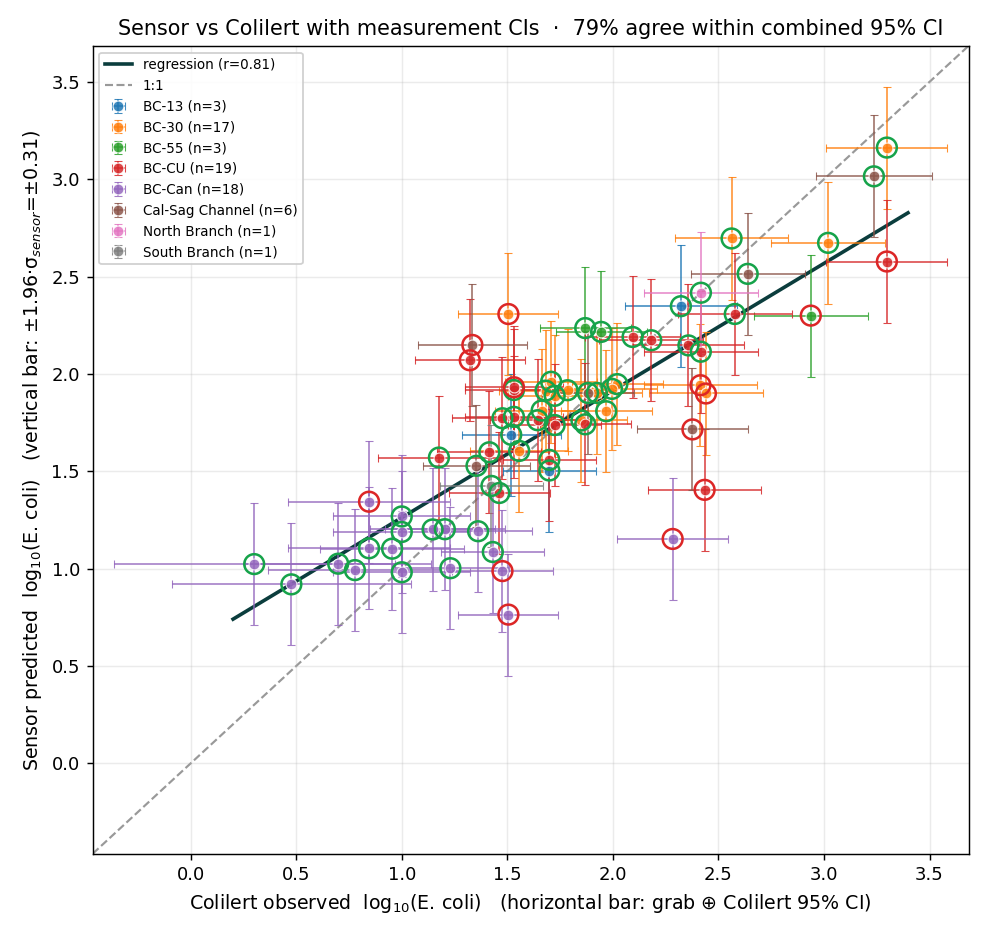
Colilert CI source: the IDEXX Quanti-Tray/2000 MPN table with 95% confidence limits (doc 2593-00; ±≈0.18 log₁₀ near 126–200 MPN).
A note on bias
The scatter measures precision (how tightly predictions track the grabs: 82% agree within the combined 95% CI in quadrature; 88% have overlapping error bars). Bias — a systematic offset — cannot be read from the in-sample fit: the per-sensor fixed intercepts absorb the mean residual, so an in-sample bias test is uninformative. A genuine bias / equivalence test (e.g. TOST against the Quanti-Tray/2000 CI margin) requires held-out data and is deferred.
Measurement-uncertainty framework & references
Every uncertainty term above is a measurement or a published value, not an assumption:
- Sensor precision (σ = 0.16 log₁₀): reproducibility of three co-located Lume units reading identical bucket water (see the Colilert-Lab page), the instrument-precision concept of ISO 15839 / ISO 5725 [1,2].
- Grab collection (σ ≈ 0.10 log₁₀): field-duplicate reproducibility of E. coli grabs (McCarthy et al. 2008, ±33%; Harmel et al. 2016 sample-collection term) [3,4].
- Colilert assay (σ ≈ 0.10 log₁₀): the Quanti-Tray/2000 95% counting CI [5] and the laboratory-analysis term of Harmel et al. [3].
- Agreement test: a point agrees when |predicted−observed| ≤ 1.96·√(σsensor²+σref²), combining standard errors in quadrature (bar-overlap would overstate agreement): a difference test in the spirit of Bland & Altman limits of agreement [8] under the GUM uncertainty framework [9].
- Attenuated slope (0.65): because the reference grab carries error, ordinary least squares under-estimates the slope; an errors-in-variables (Deming) fit would correct it [10].
- Unresolved representativeness: short-term temporal/spatial E. coli variability is real and large but site-specific, so it is left unquantified pending high-frequency data [6,7].
- ISO 15839:2003, Water quality — On-line sensors/analysing equipment — Specifications and performance tests. iso.org
- ISO 5725, Accuracy (trueness and precision) of measurement methods and results.
- Harmel et al. 2016, Uncertainty in monitoring E. coli concentrations in streams and stormwater runoff, J. Hydrology. link
- McCarthy et al. 2008, uncertainty in field-collected E. coli data (±33%).
- IDEXX Laboratories, Quanti-Tray/2000 MPN table with 95% confidence limits (doc 2593-00). PDF
- Leecaster & Weisberg 2001, Effect of sampling frequency on shoreline microbiology assessments, Mar. Pollut. Bull. PubMed
- Boehm et al. 2007, Enterococci concentrations in diverse coastal environments exhibit extreme variability, Environ. Sci. Technol. link
- Bland & Altman 1986, Statistical methods for assessing agreement between two methods of clinical measurement, Lancet.
- JCGM 100:2008, Evaluation of measurement data — Guide to the expression of uncertainty in measurement (GUM).
- Deming / errors-in-variables regression for method comparison (e.g. Linnet 1998, Clin. Chem.).
Predictive classifier (in-sample)
The exceedance classifier thresholds the deployed continuous prediction at exc_t, the shipped operating point (79 CFU for Boulder, tuned below the 126 action limit to balance the two errors); three-level probabilities bin the prediction at 126 and 1000 CFU. n = —. In-sample. These are the numbers the deployed FIELD_MODEL.slope branch produces on the current grab master, scored through predictEcoliCfu itself rather than a re-implementation. Superseded 2026-08-21: this panel previously showed the CTLF candidate on a July snapshot of 122 grabs while its own text described a different model as deployed.
Three-category — Low (<126) · Mid (126–1000) · High (≥1000)
Overall accuracy (3-level)
—
Balanced accuracy (BA-optimal op. point)
—
Read each accuracy as a range, not a point — for three independent reasons. (1) Few exceedances. Balanced accuracy rests on only — exceedance grabs out of —, so its bootstrap 95% CI (shown in the summary above) is wide; a single decimal implies precision this many grabs cannot support. (2) The reference is itself uncertain. Colilert is an MPN with a published confidence interval, and ~20% of grabs sit close enough to the 126/1000 boundaries that their true category is ambiguous — scoring against a fuzzy truth turns a point into a band (propagating the Colilert CIs moves the headline by ≈±0.03–0.04). (3) Floor vs ceiling. How you score those boundary grabs sets a floor (the hard number: counted wrong if off) and a ceiling (the “up to … within Colilert CI” line under each card — the highest score you reach once every prediction the reference cannot prove wrong is credited). The operational value lives between them. So a headline like “balanced accuracy 0.705” is better read as “credibly ~0.61–0.78, depending on sampling and reference ambiguity” (that is the measured bootstrap interval) — and the three uncertainty sources are distinct (sampling noise, fuzzy labels, and scoring convention), so they widen the range for different reasons rather than double-counting.
Loading confusion matrix…
Overall — exceedance detection (safe vs unsafe, BA-optimal operating point)
Sensitivity
—
of true exceedances (≥126 CFU), the fraction the model flags — TP / (TP + FN)
Specificity
—
of true non-exceedances, the fraction correctly cleared — TN / (TN + FP)
Collapsing to a single safe/unsafe call at the BA-optimal operating point balances sensitivity and specificity; live numbers load below.
Confidence intervals load with the live numbers above.
| class | support | sensitivity (recall) | specificity | precision | F1 |
|---|
| Loading… |
Because this is a three-category model, sensitivity and specificity are computed one-vs-rest (each category against the other two). Sensitivity (recall): of the grabs truly in a category, the fraction the model assigns to it, TP / (TP+FN). Specificity: of the grabs not in a category, the fraction the model correctly keeps out, TN / (TN+FP). Precision: of the grabs predicted in a category, the fraction truly in it, TP / (TP+FP). F1: harmonic mean of sensitivity and precision. Macro average is the unweighted mean across the three categories. Of the two headline cards above, overall accuracy is the 3-level (Low/Mid/High) fraction of grabs whose category is correct (the confusion-matrix diagonal ÷ n), and balanced accuracy is the two-level (safe/unsafe) figure at the model’s chosen BA-optimal operating point — (sensitivity + specificity)/2, where truth is <126 vs ≥126 (the action limit) and the prediction flags unsafe at ≥88 (a buffer below 126). Overall accuracy is inflated by the dominant Low class, so balanced accuracy is the better single number; it matches the safe/unsafe summary near the top of this section. The small “up to … within Colilert CI” line under each card is a CI-tolerant ceiling: a prediction is credited whenever the grab’s Colilert 95% CI cannot call it wrong — its confidence interval overlaps the predicted category (3-level) or straddles the 126 line so the true class is unresolved (safe/unsafe). Because ~20% of grabs sit close enough to a boundary for this to apply, it is a ceiling (the reference’s own resolving power), with the hard number as the floor.
Thresholding the continuous model at an BA-optimal operating point balances the two errors (live sensitivity and specificity in the cards above) — versus the old multinomial's specificity ~0.52. Raising the threshold toward 126 buys specificity; lowering it buys sensitivity. (The 3-level macro-recall is lower because the continuous fit rounds some ≥1000 grabs down to Mid; they remain flagged as exceedances.)